In this post, we will try to understand the basic mechanism behind genetic algorithm and use it to solve the reinforcement learning problem. See below how well genetic algorithm was able to balance cartpole in the 7th episode itself without using any gradient based strategy. Check out my solution on open AI leaderboard which is currently at 4th position!
Okay, before diving deep into the GA let me answer some ifs and buts, the whys and why nots with a brief background on meta heuristic – a class to which it belongs.
Why not descent down using gradient?
Gradient descent can be the go-to algorithm if you have that most desirable continuous, differentiable, unimodal function to detect “The” optimal point but hey welcome to the real world to realise that problems are not this smooth. Given a discrete function and there goes our Mr. dependable out of the bag. Also, don’t ask me to walk the pitted path of those “locals” to reach the “global” goal with normal descent. I heard somebody mentioning NP-hard.
Of course that doesn’t imply if encountered with such patchy problem then call it a quit and thus let me introduce you to the meta world where no heuristic information is required to seek the solution.
What is Metaheuristic?
Word “meta” can be linked to some degree of randomness induced in the model. Hey, don’t be just blown away by the word random as you will witness how these randomizations itself will provide a guided search towards the best solution.
How this pool of population-based metaheuristic algorithms work?
Suppose you are provided with a problem about which you don’t have any idea and in reality, it looks like below (wow, what a nightmare):
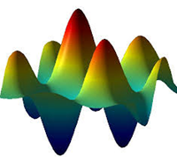
But you have this output(savior) function which returns the fitness value of your imagined solutions.
So, it starts with some random initialization (feel free to seed some points with heuristic solutions to reduce the search space but don’t dare to get rid of that rich diversity by eliminating randomness). Now, the whole exercise will reduce to exploitation versus exploration. We will select the fittest solution by exploiting the given population but also try to avoid those local traps (in case of uglier surface like above) by tweaking those individuals and exploring more surfaces. Continue till convergence or end condition.
This is the broad idea on which these population-based method are based. With this premise in mind, let’s call GA for some action.
Understanding Genetics
The name pretty much says from where it takes the inspiration but will definitely come to the fancy terminology used to describe the process. Before that an overview:
We start with initializing a pool of random solutions (consider this as selecting random vector of points on the high dimensional surface). Then, we determine the value of these random points represented in the form of weights from the available output function. Go on to select the better ones among the rest (survival of the fittest).
From the view point that new solution created will inherit better characteristic from the former ones, some information exchange takes place between the selected solutions (take it as exchanging good traits between any two solutions).
It might happen with high probability (based on the search space of initial population) that part of the space remains unexplored. This may return sub optimal solution and to ward off this fear some weights of the created solution can be tweaked to explore the unentered boundaries.
Linking above phenomena with actual terminology, we can define:
- Population – pool of individual solution.
- Child and parent – a child is the tweaked copy of a candidate solution (parent)
- Chromosome – an individual or single solution
- Genes – a particular position (point on the vector) in a chromosome
- Allele – a particular setting (arrangement of points on the vector) of a gene
- Fitness function – calculates the profit/cost (solution domain) associated with an individual
- Representation – How an individual in the population is represented internally. It can be either encoded in binary form called as Genotypic or represented as it is known as phenotypic.
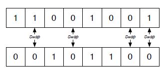
- Crossover – Swapping section of two parents to produce children (information exchange between any two individuals)
- Mutation – Randomly tweaking candidate solution (for exploration)
Pseudo Code-
- INITIALIZATION – Initialize with some random solution of population size . It can be viewed as a measure of degree of parallel search
- SELECTION – Select individuals for reproduction by giving preference to fittest individuals also viewed as selection pressure. This step can be related to exploitation phase.
- CROSSOVER – Produce offspring for next generation after tweaking selected parents. We will dig deep into types of crossover in next section.
- MUTATION – Mutate certain children to induce variation in the population. It can be linked to exploration
- Continue until certain end time/ best solution found.
Success of GAs is attributed to the phenomenon of survival of the fittest. It is proven through schema theorem stated below that fit individuals grow rapidly through generations (you can refer to Goldberg’s explanation for this).
Schema Theorem
A schema is a template that identifies similarity of string (vector of points) at certain position. High fitness vectors may contain certain pattern of points embedded at certain position.
For example, consider a length 7 schema that describes the set of all vectors of length 7 with fixed values at second, fifth and seventh position. The symbol implies that these positions can take any binary value. Also, a schema can be defined by 2 main attributes: order and defining length. The order of a schema is defined as the number of fixed values in the template, while the defining length is the distance between the first and last fixed positions. In the above example, the order is 3 and its defining length is 5. The fitness of a schema is the average fitness of all strings matching the schema. The fitness of a string is a measure of the value of the encoded problem solution, as computed by a problem-specific evaluation function.
Consider, an example of schema H at any time t given by . Since, probability of schema getting selected will be proportional to its fitness, at time we will have:
Where is average fitness of vectors with schema H at time t is average fitness of entire population. Thus, above average schema will grow and below average dies off. Assume a schema remains above average an amount . Then, we have:
Starting at 0 time, we get exponentially increasing samples for above average schemata in next generations.
If we consider crossover, then effect of disruption can be given by
being the probabilty of crossover. It can be said a schema will survive the disruption by
If probability of mutation is pm then probability of surviving mutation is given by:
For small values of , may be approximated by . Considering reproduction, crossover and mutation in the final equation:
Thus, schema theorem states that short, low order, above average schemata receive exponentially increasing trials in successive generations.
Now, let’s try to get a hang of how it works by simulating a problem of maximizing the function, where x is permitted to vary between 0 and 31. The optimal solution of this problem is 961.
#Importing Packages
import numpy as np
import random as rnd
# Always set random seeds for reproducibility
np.random.seed(0)
import matplotlib.pyplot as plt

#Importing celluloid to create animation
from celluloid import Camera
from IPython.display import HTML

def Individual(chromosome_length):
    """
    Arguments: chromosome_length - length of individual solution
    Returns: an individual solution
    Description: Here we are representing the solution in binary encoded form
    """
    ind= [rnd.randint(0,1) for _ in range(chromosome_length)]
    return(ind)

def create_population(pop_size,chromosome_length):
    """Returns: Returns a population of pop_size of indiviudal solution
    """
    pop=[]
    for i in range(pop_size):
        sequence=Individual(chromosome_length)
        pop.append(sequence)
    return(pop)

def roulette_wheel(pop):
    """
    Returns: population of selected individuals for mating
    Description: Selection is done on the basis fitness score compared to the total score of the population
    giving higher weightage to individuals with higher scores
    """
    mat=[]
    output_prob=np.array(list(map(fitness,pop)))/sum(list(map(fitness,pop)))
    for i in range(len(pop)):
        idx=np.random.choice(range(len(pop)),1,p=output_prob)
        mat.append(pop[idx[0]])
    return(mat)

def one_crossover(parent_1, parent_2):
    #use one point crossover to combine two parents to create two children

    chromosome_length = len(parent_1)
    crossover_point = rnd.randint(1, chromosome_length-1)
    child_1 = []
    child_2 = []

    child_1.extend(parent_1[0:crossover_point])
    child_2.extend(parent_2[0:crossover_point])
    child_1.extend(parent_2[crossover_point:])
    child_2.extend(parent_1[crossover_point:])

    #mutate children
    mutate(child_1, mutationRate)
    mutate(child_2, mutationRate)

    return child_1,child_2

#randomly mutate a solution for exploration
def mutate(individual, mutationRate):
    for swap in range(len(individual)):
        if(rnd.random() < mutationRate):
            individual[swap] = 1-individual[swap]
    return individual

def generations(episodes,pop,mutationRate):
    """    Arguments: episodes - Number of generations for which iteration wil continue to find optimal solution
               pop - Number updates to the policy
               mutationRate - mutation probability
    Returns: an animation object
    Description: Individuals are updated in each generation to return the optimal solution
    """
    fig = plt.figure()
    # Setting up camera to capture frames for animation
    camera = Camera(fig)
    for i in range(episodes):

        #individuals with higher fitness score are selected with higher probability for breeding
        mating=roulette_wheel(pop)
        children=[]
        for j in range(int(len(mating)/2)):

            #crossover and mutation is performed on selected individuals
            child_1,child_2=one_crossover(mating[j],mating[len(mating)-j-1])
            children.append(child_1)
            children.append(child_2)
        pop=children
        plt.plot(x,x**2 ,color="b")
        plt.plot(np.sqrt(np.array(list(map(fitness,pop)))),np.array(list(map(fitness,pop))),marker='o',
                 color='r',markersize=12)
        camera.snap()
    plt.close()
    return camera

mutationRate=0.02
#create a population of size 6
pop=create_population(6,5)
camera = generations(20,pop,mutationRate)
animate = camera.animate()
HTML(animate.to_html5_video())
Short, low order and highly fit schemata are sampled and recombined to form high performing solutions (as they grow exponentially) instead of trying every possible combinations. We try to generate better and better solutions from the best partial solutions of past samplings. We can carry some top performing solutions to other generations known as elite solutions without any tweaking so that to avoid skipping optimal solution due to too much exploration.
Brief description of operators
Let’s cover some common operators used with python implementation of how reinforcement learning problem can be solved using this algorithm.
For solving the cartpole, a simple 2 layered neural net was created which is used for initialization. Population of size “num_agents” is generated using this net to initialize agents with different weights.
def population(num_agents):

    agents = []
    for _ in range(num_agents):
        #Class LunarLander(neural net) is called to initialize weights of agents
        agent = LunarLander().to(device)

        for param in agent.parameters():
            param.requires_grad = False

        agents.append(agent)

    return agents
Techniques for selecting fittest individuals for breeding:
Roulette Wheel or fitness proportionate –
In this, individuals are selected based on fitness compared to average fitness of the population. The probability of selecting an individual can be given by:
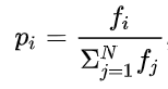
It is equivalent to rolling a roulette wheel (completely a casino thing). All non-casino folks out there, don’t feel left out, here is a quick help. Basically, there is a fixed point/arrow and a wheel (how subtle!) which is rotated and individual corresponding to the point where it stopped stands selected.
To execute this, we proceed in a following manner:
- Do a cumulative sum of probabilities for all individuals
- Generate a random no. between the range 0 to 1 and individual falling in the produced range is selected for next generation.
It works well in the initial iterations when there is significant difference between individuals but possesses a disadvantage of not being able to distinguish between individuals when fitness becomes similar in later generations.
Stochastic Universal Sampling-
A version of fitness proportionate with only difference of multiple fixed points spaced evenly to select individuals unlike conducting repeated sampling in case of the former one. It gives chance to weaker solution as well to get selected.
Rank Selection-
It sorts the individual according to the fitness score and selects top performing individual. Thus, it is able to distinguish between individuals when fitness becomes similar but can be computationally expensive due to sorting algorithm used.
I used rank selection to create mating population by sorting individuals on the basis of mean rewards (10 parallel environment was created to compute mean reward for each agent).
def rank_selection(agents, sorted_parent_indexes,cross):
    """Select individuals for reproduction by giving preference to fittest individuals
    """
    children_agents = []

    for i in range(cross):
        selected_agent_index = sorted_parent_indexes[np.random.randint(len(sorted_parent_indexes))]
        children_agents.append(agents[selected_agent_index])
    return children_agents
Tournament Selection-
This technique is popular nowadays as it possesses less computational complexities and has an added advantage of performing at par with linear ranking without having to sort population on the basis of fitness. In k-way tournament selection, for each selection k individuals are randomly selected and then one with the best fitness is selected. Basically, conducting fight among k individuals and choosing the best among them.
Why do we need crossover?
In a way, information of important traits get dispersed in the population to create more high performing samples. Below are some crossover techniques that can be used to carry out disruption:
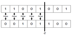
1-point crossover-
A position is randomly selected on the vector and values are swapped for a broken segment.
Thinking in terms of schema, 1-order samples won’t be affected by this disruption. But higher order samples will be affected but not with same probability. Consider 2 schemata:
- probability that bits in this schema will be disrupted is 1/L-1
- probability that bits in this schema will be disrupted is L-1/L-1 or 1
Therefore, position of the bits matter when using 1-point crossover. Thus, correlated bits located at large distance will be separated with higher probability.
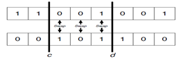
2-point crossover-
A special case of 1-point crossover where 2 points are selected randomly to carry out the bit transfer. It could be less disruptive compared to 1-point as vector can be visualized in the form of a rings so bits at extreme ends will not likely be disrupted.
For 1-point and 2-point crossover, schemata which have bits that are close together on the vector are less likely to be disrupted by crossover.
Uniform Crossover-
This operator does not put limitation of defining length between the bits as positions for swapping bits are randomly selected in this case. This means that each bit is inherited independently from any other bit and that there is no linkage between bits.
In general, the probability of disruption is , where o(H) is the order of the schema.
In research, it is suggested that probability of disruption for uniform crossover is greater than the rest of the two operators but still it sometimes performs better especially for smaller population.
In this example uniform crossover is used in which probability of crossover is decayed through generations (given by uni_prob).
def uniform_crossover(ind1,ind2,layers,uni_prob,mut_threshold):
    """
    input: ind1,ind2 - parents between whom crossover is to be performed
           layers - total layers in the neural net * 2(to account for the bias)
           uni_prob - probability for uniform crossover
           mut_threshold - probability for mutation
    returns tweaked copy of parents
    """
    offspring=[]
    for i in range(layers):
        dim=list(ind1.parameters())[i].shape
        idx=torch.randperm(int(np.prod(dim)*uni_prob)).reshape(1,-1).to(device)
        list(ind1.parameters())[i]=list(ind1.parameters())[i].reshape(1,-1).scatter_(1,idx,list(ind2.parameters())[i].reshape(1,-1)).reshape(dim)
        list(ind2.parameters())[i]=list(ind2.parameters())[i].reshape(1,-1).scatter_(1,idx,list(ind1.parameters())[i].reshape(1,-1)).reshape(dim)
    sample = rnd.random()

    if sample<0.4:
        ind1=mutate(ind1,mut_threshold)
        ind2=mutate(ind2,mut_threshold)
    offspring.extend((ind1,ind2))
    return offspring
Mutation
An individual can be randomly tweaked in order to enable exploration in the population. Below is the case wherein we are exponentially decaying the mutation threshold through generation such that in initial phases greater exploration is there and in later phases we decrease the probability.
def mutate(agent,eps_threshold):
    """
    input: individual to be mutated and threshold by which each weight will be mutated
    returns mutated individual
    """

    child_agent = copy.deepcopy(agent)

    mutation_power = eps_threshold

    for param in child_agent.parameters():

        if(len(param.shape)==2): #weights of linear layer
            for i0 in range(param.shape[0]):
                for i1 in range(param.shape[1]):
                    if rnd.random()<0.6:
                      param[i0][i1]+= mutation_power * np.random.randn()


        elif(len(param.shape)==1): #biases of linear layer or conv layer
            for i0 in range(param.shape[0]):
                if rnd.random()<0.6:
                  param[i0]+=mutation_power * np.random.randn()

    return child_agent
Below is the main snippet that calls all the function to run through the generations. You can click here! to see the full code.
 game_actions = 2 #2 actions possible: left or right
#disable gradients as we will not use them
torch.set_grad_enabled(False)

# initialize N number of agents
num_agents = 150
n_elite=5

agents = population(num_agents)
# # How many top agents to consider as parents
top_limit = 20
# # # run evolution until X generations
generations = 500

#threshold decay for crossover
EPS_START = 0.6
EPS_END = 0.2

steps_done=0

#mutation threshold is exponentially decayed from 0.9 (higher exploration) to 0.01 in later generations
MUT_START = 0.90
MUT_END = 0.01
EPS_DECAY = 200
cross=round(num_agents*0.7/2)*2
mut=num_agents-cross
scores=[]

for generation in range(generations):
    # return rewards of agents
    rewards=list(map(fitness,agents))
    sorted_parent_indexes = np.argsort(rewards)[::-1][:top_limit]

    eps_threshold = EPS_END + (EPS_START - EPS_END) * \
    math.exp(-1. * steps_done / EPS_DECAY)

    mut_threshold = EPS_END + (MUT_START - MUT_END) * \
    math.exp(-1. * steps_done / EPS_DECAY)

    #select children for breeding
    mating=rank_selection(agents, sorted_parent_indexes,cross)
    children=[]
    for j in range(int(len(mating)/2)):
        #perform crossover of 70% population
        child=uniform_crossover(mating[j],mating[len(mating)-j-1],4,0.2,eps_threshold)
        children.extend(child)

    #only mutate 30% of the population
    children_agents=return_mutation(agents, sorted_parent_indexes,n_elite,mut,mut_threshold)
    children=children_agents+children

    top_rewards = []
    for best_parent in sorted_parent_indexes:
        top_rewards.append(rewards[best_parent])

    agents=children
    print("Generation ", generation, " | Mean rewards: ", np.mean(rewards), " | Mean of top 5: ",np.mean(top_rewards[:5]))
    print("Rewards for top: ",top_rewards)
    scores.append(top_rewards[0])
    if len(scores) >= 100:
        if np.mean(scores[-100:]) >= 195.0:
            print('Solved after' + str(generation-100) + ' episodes')
            break
    steps_done+=1
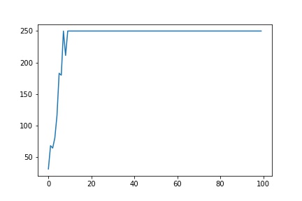
CartPole defines “solving” as getting average reward of 195.0 over 100 consecutive trials. It can be seen in the above plot that we were able to solve the problem in 7th episode itself.
Go ahead and tweak the code to solve other reinforcement problems as well.
References:
Evolutionary Computing/Metaheuristics images in this post are snipped from this book